![](https://cplab.blog/wp-content/themes/cocoon-master/images/b-woman.png)
前回までは、データの確認を行いました。
今回からいよいよ機械学習をさせます!
![](https://cplab.blog/wp-content/themes/cocoon-master/images/b-man.png)
AIを作る肝の部分ですね!
ついていけるように頑張ります!
機械学習とは
![](https://cplab.blog/wp-content/themes/cocoon-master/images/b-woman.png)
機械学習を実際に行う前に、機械学習について理解しましょう。
![](https://cplab.blog/wp-content/themes/cocoon-master/images/b-man.png)
お願いします!
![](https://cplab.blog/wp-content/themes/cocoon-master/images/b-woman.png)
「機械学習」とは、「機械(コンピュータ)が自動で学習し、データに関する法則やルール、パターンを見つけ出す方法」のことです。
![](https://cplab.blog/wp-content/themes/cocoon-master/images/b-man.png)
コンピュータが自動で学習するのですか?
凄いですね!
![](https://cplab.blog/wp-content/themes/cocoon-master/images/b-woman.png)
機械学習には、教師あり学習と教師なし学習、強化学習の3種類があります。
![](https://cplab.blog/wp-content/themes/cocoon-master/images/b-man.png)
それぞれどういう違いがあるのですか?
![](https://cplab.blog/wp-content/themes/cocoon-master/images/b-woman.png)
教師あり学習とは、学習データに正解を与えて学習させる方法です。
教師なし学習とは、学習データに正解を与えずに学習させる方法です。
強化学習とは、スコアの最大化を目標として行動を学習させる方法です。
![](https://cplab.blog/wp-content/themes/cocoon-master/images/b-man.png)
今回の手書き数字の学習はどれにあたるのですか?
![](https://cplab.blog/wp-content/themes/cocoon-master/images/b-woman.png)
今回の学習は、教師あり学習にあたります。
手書き数字のデータに、これは「3」ですなどの正解を与えて学習させるからです。
![](https://cplab.blog/wp-content/themes/cocoon-master/images/b-man.png)
そうなんですね!
- 機械学習=機械(コンピュータ)が自動で学習し、データに関する法則やルール、パターンを見つけ出す方法
- 機械学習には、教師あり学習、教師なし学習、強化学習の3種類がある
- 教師あり学習=学習データに正解を与えて学習させる方法
- 教師なし学習=学習データに正解を与えずに学習させる方法
- 強化学習=スコアの最大化を目標として行動を学習させる方法
実際に機械学習させてみよう
![](https://cplab.blog/wp-content/themes/cocoon-master/images/b-woman.png)
では、いよいよ機械学習をさせてみましょう!
ファイル「ml」を作成して、以下のコードを実行してください。
# 手書きの数字のデータを読み込む
from sklearn import datasets
digits = datasets.load_digits()
X = digits.images
y = digits.target
X = X.reshape((-1, 64))
# データをトレーニング用とテスト用に分ける
from sklearn.model_selection import train_test_split
X_train, X_test, y_train, y_test = train_test_split(X, y, test_size = 0.2, random_state = 0)
# データを学習
from sklearn.naive_bayes import GaussianNB
classifier = GaussianNB()
classifier.fit(X_train, y_train)
# 予測して精度を見る
from sklearn import metrics
from sklearn.metrics import accuracy_score
y_pred = classifier.predict(X_test)
print(accuracy_score(y_test, y_pred))
![](http://cplab.blog/wp-content/uploads/2022/06/スクリーンショット-2022-06-06-22.58.23-1024x484.png)
![](https://cplab.blog/wp-content/themes/cocoon-master/images/b-man.png)
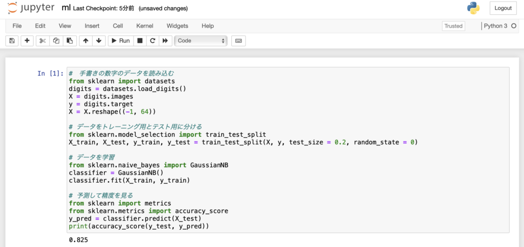
「0.825」という数字が出てきました!
![](https://cplab.blog/wp-content/themes/cocoon-master/images/b-woman.png)
よくできました!
では、コードの解説をしていきます。
ブロックごとに開設していきますね。
![](https://cplab.blog/wp-content/themes/cocoon-master/images/b-man.png)
よろしくお願いします!
![](https://cplab.blog/wp-content/themes/cocoon-master/images/b-woman.png)
まず、1つ目のブロックですが、データの読み込みを行う部分です。
「from sklearn import datasets」でdatasetモジュールを読み込んで、
「digits = datasets.load_digits()」で手書きの数字のデータを読み込みます。
![](https://cplab.blog/wp-content/themes/cocoon-master/images/b-man.png)
ここまでは前回までにやったことですね!
![](https://cplab.blog/wp-content/themes/cocoon-master/images/b-woman.png)
はい!
そして、Xを手書きの数字の画像を、yに手書き数字の画像の答えを定義します。
![](https://cplab.blog/wp-content/themes/cocoon-master/images/b-man.png)
なるほど。
![](https://cplab.blog/wp-content/themes/cocoon-master/images/b-woman.png)
そして、最後に、「X = X.reshape((-1, 64))」で二次元配列を一次元配列に変換します。
これはどういうことかというと、画像データを一次元の情報にして、機械学習をしやすいようにします。
![](https://cplab.blog/wp-content/themes/cocoon-master/images/b-man.png)
画像データだと機械学習がしにくいので、一次元配列に変換するんですね。
![](https://cplab.blog/wp-content/themes/cocoon-master/images/b-woman.png)
そして、次のブロックでデータを学習するための分と、テストを行うための分に分けます。
「from sklearn.model_selection import train_test_split」でtrain_test_splitモジュールを呼び出して、次の行で、データを実際に学習する分とテストする分に分けます。
次の文の中に「test_size = 0.2」と書いてあるとおり、テストする分のデータが全体の2割になるように分けます。
![](https://cplab.blog/wp-content/themes/cocoon-master/images/b-man.png)
ということは、学習する分のデータは8割になるわけですね。
![](https://cplab.blog/wp-content/themes/cocoon-master/images/b-woman.png)
その通りです!
そして、「random_state = 0」と書くことで、データの分割結果が固定されます。
つまり、書かない場合は、実行するたびにデータの分割結果が毎回異なることになります。
![](https://cplab.blog/wp-content/themes/cocoon-master/images/b-man.png)
そういうことだったんですね。
![](https://cplab.blog/wp-content/themes/cocoon-master/images/b-woman.png)
次のブロックに行きます。
次のブロックでいよいよデータを学習させます。
今回は、「ナイーブベイズ」というアルゴリズムを使って学習させました。
「from sklearn.naive_bayes import GaussianNB」でアルゴリズムを読み込み、
「classifier = GaussianNB()」でアルゴリズムを定義します。
そして、「classifier.fit(X_train, y_train)」で学習します。
![](https://cplab.blog/wp-content/themes/cocoon-master/images/b-man.png)
たった3行で学習できるなんてすごいですね!
![](https://cplab.blog/wp-content/themes/cocoon-master/images/b-woman.png)
そして、最後のブロックで評価します。
「from sklearn import metrics」「from sklearn.metrics import accuracy_score」で評価に必要なモジュールを読み込みます。
次に、「y_pred = classifier.predict(X_test)」でテストデータを使って、予測を行います。
最後に、「print(accuracy_score(y_test, y_pred))」でテストデータと予測データを用いて「正解率」というものを求めます。
![](https://cplab.blog/wp-content/themes/cocoon-master/images/b-man.png)
正解率とはどうやって求めるのですか?
![](https://cplab.blog/wp-content/themes/cocoon-master/images/b-woman.png)
正解率は、「正解数/問題数」です。
![](https://cplab.blog/wp-content/themes/cocoon-master/images/b-man.png)
すなわち、今回の場合の正解率が「0.825」ということですね。
![](https://cplab.blog/wp-content/themes/cocoon-master/images/b-woman.png)
その通りです!
![](https://cplab.blog/wp-content/themes/cocoon-master/images/b-man.png)
ということは、高い正解率が得られたということですね。
![](https://cplab.blog/wp-content/themes/cocoon-master/images/b-woman.png)
そうですね。
でも、もしかしたら、もっと高い正解率が得られるアルゴリズムがあるかもしれません。
次回は、「SVM」というアルゴリズムで学習させてみましょう。
![](https://cplab.blog/wp-content/themes/cocoon-master/images/b-man.png)
分かりました!
- まず、最初にデータを読み込む
- 次に、データを学習用とテスト用に分ける
- データを分けたら、学習させ、学習モデルを構築する
- 構築した学習モデルを用いて予測し、「正解率」の指標を用いて評価を行う
まとめ
![](https://cplab.blog/wp-content/themes/cocoon-master/images/b-woman.png)
今回は、機械学習を実際に行ってみました。
![](https://cplab.blog/wp-content/themes/cocoon-master/images/b-man.png)
思っていたよりも簡単でしたね。
![](https://cplab.blog/wp-content/themes/cocoon-master/images/b-woman.png)
そうですね。
基本的には、
①データを読み込む
②データを学習用とテスト用に分ける
③学習
④予測して評価
の4段階で機械学習ができます。
ぜひ覚えておいてくださいね!